Combusion Model: A reactive flow model
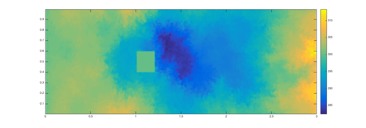
Figure 1: Temperature contour with \( Re=\infty \) at the end of the simulation time (\(\frac{tU}{H} = 90 \)).
In this project, a simple premixed combusion numerical model is implemented in addtion to our Navier-Stoke solver to observe the interaction of liquid
atomization and spray vaporization in a heat combustion process as the fuel consumed by the flame. A reactive flow in an augmentor with a mixture of
fuel and oxidizer flows in the turbine exit channel is modelled. A box is used as a flame-holder to create a low-speed region to stablized the flame.
Simulation results:
The combustion model is described by the following equations:
$$ \frac{\partial \phi}{\partial t} + \nabla \cdot \left( u \phi \right) = \mathcal{D} \nabla^2\phi + \dot{\omega_{\phi}} $$
and
$$ \frac{\partial T}{\partial t} + \nabla \cdot \left( u T \right) = \mathcal{D} \nabla^2\phi + \dot{\omega_{T}}. $$
where \( \phi \) represents the amount of combustible material avaliable and \( T \) represents the temperature.
In these, the combustion source terms are taken to be
$$ \dot{\omega_{\phi}} =-\dot{\omega} $$
and
$$ \dot{\omega_{T}} =A\dot{\omega} $$
where we consider the following Arrhenius reaction
$$ \dot{\omega}= \phi \left( \frac{T}{T_b} \right)^3 e^{\frac{- T_a}{T}}. $$
In the above expressions, \(\mathcal{D}=10^{-4}\), \(A=1000\), \(T_a = 1500\), and \(T_b = 1000\). As initial conditions, we have an \(H \times H\) region behind the square obstruction where \(T=2500\).
The viscous term in the Navier-Stoke is solved implicitly through the Crank-Nicolson scheme with alternating direction implicit (ADI) method. The combustion equations are solved using second order accuracy in time ( \( \textit i.e. \) Adams-Bashforth for convection and Crank-Nicolson with ADI for diffusion), second order central differencing in space for the diffusion term, and third order QUICK for the spatial discretization of the convective term.
The convergence criterion for the simulations is set to \(\epsilon = 10^{-10}\) with maximum subiteration \(iter_{max} = 1000\). The total simulation run time is \(\frac{tU}{H} = 100 \).
Video 1: Temperature contour with \( Re=1000 \).
Video 2: Velocity contour with \( Re=1000 \).
Video 3: Temperature contour with \( Re=\infty \).
Video 4: Velocity contour with \( Re=\infty \).